2017-02-22

Exploring data with Visual Studio Code

Fig 1: Visual presentation of Radix sort steps
Every now and then I have a need to visualize some data, be it spectral spread of stars in a cluster, a spurious correlation or a stream of measurements. I've always used whatever happens to be handy and available, often kludging data from format to another and using Excel or Python+matplotlib to create the visuals. Both have repeatedly left me wanting on either appearance or ease of updating.

Enter Visual Studio Code to the equation. A small, nimble editor with interesting extensions: Python with support for Jupyter notebooks and Bokeh chart library. And the best part is, Python and Jupyter notebooks are first class citizens in the big data cloud services. So I should be able to take my existing code, update data reading parts to read my data points from cloud storage and I'd be ready to marvel a beautiful visualization of said data in my browser.

Installing tools

To start on the journey, you need to install a few things. To start, install Visual Studio Code first. And you need to install Python, I recommend 3.6.0 and the libraries for number crunching and visualization. You can use PIP for that on command line, i.e. use either pip install <package_name> or  python -m pip install <package_name>

Python Packages you need are:
Fig 2: Visual Studio Code extension for python
  • numpy
  • scipy
  • bokeh
  • jupyter
  • ipython
  • pylint
Optional but nice to have libraries are:
  • matplotlib
  • pandas
Some libraries might be included already as dependencies of the others. Now you are almost ready to go, so start up VSCode and go to the extensions tab and search for "Python" (see Fig 2). Install and reload the VSCode window.

First chart

To test everything works, you need a simple test case, how about a simple parabolic curve?
Fig 3: Code and output for a simple chart

So, what's going on there? The line 2 contains a IPython notebook cell separator, you can use these to mark executable cells for your notebook, and click on the "Run cell" button above marker to execute the following block of code. Read more on a Jupyter notebooks on VSCode by the author of the Python extension, Don Jayamanne.

The lines 3-6 import several Python module, namely Bokeh features for outputting to a notebook, plotting a figure and displaying inline-HTML text.

The line 8 defines a dictionary of common parameters for our plots, these get used by the kwargs syntax when calling plot().

Line 9 defines that our output should be a notebook and it should use inline resources instead of network resources.

Line 10 creates a sample text output to our notebook.

Lines 11-13 create a data set and a plot for it.

Line 14 shows our plot on the notebook.

Line 15 ensures that the notebook is pushed into VSCode output window.

More charts

Let's try a bigger sample, showing how a radix sort changes the array in each iteration.


The output can be seen in Fig 1. This code uses Numpy to create an array of random numbers, then sorts those using an implementation of radix sort in base 16. The interim sorting round arrays are plotted to a single figure using the multi_line -function.

If you want even more, you can take a look at the Bokeh examples, such as Heatmap.py which creates an HTML file with charts and opens it into your browser. A good excercise is to update that code to output into the VSCode window instead.

Issues

At least currently there are a few glitches. The Python kernel isn't keen to change the output method of Jupyter notebooks, so if you have multiple windows open with both HTML file and VSCode window output, your HTML files might get corrupted when executing a cell from another file. To get around this, point your mouse to the status row at bottom, click on the "Python 3 kernel" and select "Restart Python 3 kernel" whenever switching between files. I haven't found a direct Shift-Ctrl-P shortcut command for this yet.
2015-01-17

Astrophysics as a side-product

Messier 48
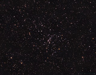
LRGB image of Messier 48 taken in April 2013
I ran across a forum posting on creating Hertzsprung-Russell diagrams from astrophotos using PixInsight. Since PixInsight is my tool of choice for processing astronomical data, I decided to try it out on one of my image stacks.
The process itself is quite straight forward as described. Once images are calibrated, registered and stacked, you simply generate CSV files from V and B channels (green is close to photometric V) using the FWHMEccentricity script in PI. From my image it found 1266 stars for G and 836 for B.
For reference data on actual magnitude you then solve the image and use AnnotateImage to generate a file containing Tycho catalog data on found stars (found 241).

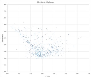
M48 Hertzsprung–Russell diagram
Hertzsprung-Russell diagram of Messier 48 with 809 stars
The three generated files are combined on spreadsheet, the star fluxes are calculated from the FWHM data
Flux=(A*SizeX*SizeY*Pi/3)
and all stars on all files get a positional index
Index= int(X)+int(Y)*ImageWidth
that is later used to correlate individual stars. If you use Excel, put Index into column A. The flux is converted to magnitude scale with
mag=-2.5 * Log10(flux)

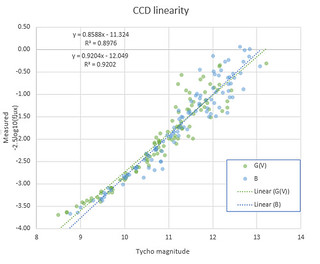
M48 HR data linearity
SXVR-H18 CCD linear fit shows anti-bloom gate effect on the brighter stars bottom-left
Now we have all the datapoints in compatible numeric spaces, so the calculated magnitudes can be fitted with catalog data using a simple linear regression. In Excel you can use VLOOKUP macro to match each star by the calculated Index to match the across the three files. Create separate fits for V (or G) and B, and use the fit function to create yet another column for linearized magnitudes. You can also simplify this by simply using the average offset, if your linear fit is very good and the channel fit slopes nearly identical.

Once you have your calibrated magnitudes from your image data, you can create the final column, "B-V" and use it with V (or G) to create a scatter plot. Put V as the vertical axis and reverse the axis to increase downwards. Clamp the ranges, adjust styles and enjoy your newly generated (pseudo)science. If all goes well, you should be able to see a plot that matches some region of the real star sequence plots. My M48 seems to be a pretty good match on main sequence and sub-giant stars.

2013-09-25

Update on shutter repairs

After a serious series of testing the refurbished shutter modules I have learned more. There's another way for the shutter to fail, and it's sneaky. The shutter blades are very thin metal and they very quickly gnaw a bit of play around the slotted axel. There's also some slack on the planetary gear, and as a result the shutter can flop about a minute amount. The movement is very minimal, but with relatively small tolerance that's enough to cast a shadow on the edge of sensor, or have a tiny gap when closed. I wouldn't have noticed this less I had held the assembled camera in hand and looked in with the camera at the right angle. I tried a range of glues, but those didn't hold on the blade and tiny axel at all. I was running out of options when I realized the play isn't an issue, all I have to do is make sure the blades don't flail around out of position. The easiest way was to make a miniscule wavy bend on the shutter blades, so the friction of the shutter sandwich is just enough to resist the gravitational pull on the blades. After some trial and error on the test-rig I finally ended up with a friction brake that didn't hinder shutter movement even at the low-energy 2.5V 60mA pulses, yet prevented the blades from changing their angle on their own. As luck should have it, it's a clear night tonight. And not a single shutter failure, yet.

2013-09-20

Shutter repairs


Testing a shutter
The full-sized image has lots of annotations for you to check out.
The shutter on my SXVR-H18 CCD-camera broke after three years of use, so I e-mailed the manufacturer to order one or two shutter modules as spare parts. Unfortunately they didn't have any in stock, but a day or two later I received an email saying I've been sent a box with a few old shutter modules in an unknown condition. That box arrived today in a thoroughly crushed shape, containing five nearly intact shutter modules in plenty of bubblewrap. They were apparently from various stages of manufacturing as they were all fairly different. The structure was the same in all (obviously, as they are for the same camera) but the electronics (current limiters and a parallel caps), shutter blades and mechanism substrates were all different among the modules. This was going to be fun.

I made a small 2-pin test-harness for the motor power connector to check the electro-mechanics, quickly tested all modules and none worked properly (could be from the rough handling of the package). So I disassembled all the shutters and sorted the parts based on condition. After the sorting thru the pieces I came out with three busted motors (two are needed per shutter), three pairs of warped, uncoated shutter blades and three working shutter.I had enough one the good parts pile to build at least one, most likely three, possibly even four working shutters modules. I decided to build three as making the fourth would require a bit more tools than I had taken out for the job.

The test-rig for the assembled shutter-modules was rather simple and I didn't even take a picture of it. Just a wide rubber band (visible in above image, too) to keep the shutter from over-extending and the same 2 pin connector for power from the bench supply as for motor tests. Tapping the pin-header on the shutter opens or closes the blades depending on polarity, and the motion stops against the rubber band.

The image is from testing one of the refurbished shutter modules on the camera (I should probably cut a smaller bit of antistatic mat for the computer desk as well to be on the safe side). Although all three were just fine with my test-rig, at first only one of those worked on the camera it self. Once I re-measured a rough estimate on the actual camera shutter signal, I lowered my test-rig voltage to 2.5V and limited the current to 60mA. With these I was able to repeat the performance on camera, and an hour or two later I finally had three fully functional shutter modules.

Out of curiosity I check the failed motors in more detail. The motors are small, 6mm diameter DC-motors with an equally tiny planetary gearbox. A shutter blade is press-fitted on the output shaft. Two of the broken motors were burnt or stuck and didn't turn at all, and the motor from my camera had it's planetary gearbox shred to powder, but the motor itself works just fine. I guess the cold winter nights can have an effect on polymers and they simply can't take the stress at low temperatures (below -30°C on clear winter nights).

In theory I should be able to rebuild one more shutter when the current installed one fails, and if these last at least a season each I should be OK till a proper replacement for the KAF-8300 sensor arrives. My requirements for a replacement are quite simple: no mechanical shutter, same diagonal or more, roughly the same pixel size. And a backlit sensor with better QE, especially on Ha-band, would be nice.

Now all that's left to do is to get a small bottle of argon, go to a clean place, recall how to completely clean a CCD-sensor, re-dry the humidity eaters and reassemble the camera in an argon-bath, so I don't have to worry about sublimated ice on the sensor surface.

2013-09-08

I never bin my color channels more than luminance

And here's why: When you're working on an LRGB image set, many frequently stack the images channel by channel, and then combine the RGB to chrominance and L to luminance. In doing so, you're throwing away good luminance data.

With most of the LRGB filter sets the Red, Green and Blue filters cover combined nearly the exact bandwidth of the Luminance filter. So exposing the same duration at same binning on all filters means I can sum each RGB sequence to an additional L frame, and I've "wasted" only two frames' worth of exposure time from luminance data. If I shot the RGB with a higher binning and different exposure, all that time would be wasted from luminance and my color channels would be crappier due to worse spatial resolution.

Binning your color channels is beneficial only when you have really dark skies and the sky noise doesn't drown out the read-noise with any sensible exposure durations. If your luminance exposures are easily longer than sky limited color channels at 1x1 binning, you are wasting time and resolution by binning the colors. There's no need to expose at the shortest possible sky-limited times, it should be considered the minimum exposure time, and the maximum exposure time is set by saturation of your target on sensor.

As a case study, below are two full-resolution crops of the same spot in my M31 mosaic showing the difference. The mosaic is a 2 by 2 panels, each panel is made from 10 minute exposures, 6 for L and 5 for RGB each.

Stack of six 10 minute luminance frames
Stack of same 6 luminance frames and 5RGB-sums.
As you can see, the stack of only L frames is a fair bit noisier, and it has a faint satelite streak going thru as there wasn't enough data to weed out all traces of it.

For the lower image, each RGB-set was summed as a synthetic luminance frame, and these 11 luminance frames were stacked for the final image. Some care must be take of course, don't normalize your RGB frames when calibrating, that could throw you data a bit off.

Some image processing (like PixInsight) allow you to weight the combination based on noise modelling. This does seem to return a decent approximate of a sum, if you have normalized the color frames during calibration.


2013-04-22

Season Finale

The end of another astrophotography season has come and passed. I managed to shoot two more targets on the last night of astronomical darkness of the 2012-2013 imaging season. The moon-lit astronomical darkness lasted for a whopping 14 minutes, the next few dark minutes are due in late August. The moon was at 70% full, but as most of the snow had melted the sky bacground brightness was pretty OK, it stayed level for about an hour on both side of proper midnight.


Season Finale
Originally uploaded by Mickut
The comet C/2011 L4 PANSTARRS has moved way up north. It was roughly half way up between Shedir and Caph (the two "right-most" stars in Cassiopeia's W-shape).

Due to it's northern position and the poor visibility north, I was able to image this only for half an hour in the waxing twilight before the comet was obscured by trees. With an hour or two more I might have been able to get a bit better stars on the background as the comet would have moved further during the stack.

LRGB 9x 1 minute per channel, double stacked (comet + stars).


Messier 13
Originally uploaded by Mickut
The very last deep sky image on the 2012-2013 astrophotography season was the Messie 13, a large globular cluster in Hercules. The image is stacked from six 5 minute exposures with LRGB filters. This does kill a bit of the interesting bits in the center, but brings out a lot of background galaxies.

2013-03-17

Bode's nebula and friends


Bode's nebula and friends
Originally uploaded by Mickut
A rare streak of several clear nights in a row just after new moon gave me an opportunity to expose fairly deep in all channels. I have in total almost 40 hours of exposures for this target with Luminance, Red, Green, Blue, SII, Ha and OIII filters, so future renditions with different combinations are possible in the future.

Via Flickr:
The Bode's nebula (Messier 81, which is actually a grand spiral galaxy), the Cigar galaxy (Messier 82) and NGC 3077 in a family portrait. Seen around the galaxies, but much closer, is faint dusty wisps from our galaxy the Milky Way, in the form of Integrated Flux Nebula illuminated by all the Milky Way's stars.

This image is an enhanced color image, combining "traditional" LRGB data augmented with narrowband Ha, SII and OIII emission bands. I wanted to keep the colors quite natural, so as the narrowband emissions not to overpower the scene.

Per channel exposures:
L: 39x10min
R: 33x10min
G: 32x10min
B: 32x10min
Ha: 15x30min
SII: 8x30min
OIII: 7x30min

Total integration time 37 hours 40 minutes